Project · generative models for RF

Antenna Array Failure Compensation via Constrained Conditional Flow Matching

A phased-array antenna is a row of little emitters whose signals add up in the air. Get the amplitudes and phases right and the sum is a sharp beam with quiet sidelobes. Kill a quarter of the elements and the beam smears, the nulls fill in, the sidelobes climb. Can you retune the survivors to rebuild the pattern you wanted — knowing only the target pattern and which elements are dead?

This is a full write-up of a project I built end to end on a MacBook: the physics forward model, a dataset of a hundred thousand repair problems, three families of solver, and a constrained conditional flow-matching model that samples working fixes in one shot with the antenna physics baked into every step. I’ll define the problem precisely, explain each method, describe the experiments, show the results, and analyze what they mean.

0.41°

beam-pointing error, CFM (vs 19–33° for baselines)

0

constraint violations, by construction

82%

of hard cases yield ≥2 distinct valid fixes

1e‑6

forward model vs. analytic ULA

1 · The problem, precisely

Take a uniform linear array (ULA): N = 32 isotropic elements on a line, half-wavelength spacing. Element n carries a complex weight wₙ (an amplitude and a phase). The far-field array factor — the pattern radiated toward direction θ — is a weighted sum of steering phases:

AF(u) = Σ_n w_n · exp(j · 2π · d · p_n · u),   u = sin θ,   d = 1/2 On the fixed 256-direction grid, this becomes one complex matrix multiply: A·w.

A healthy array with uniform weights gives the familiar sinc-like beam with a −13.26 dB first sidelobe.

Now a set of elements die: their weights are forced to exactly 0. We are given

• a target pattern — the desired far field, as magnitude only (20·log₁₀|AF| in dB), because that is what you actually measure or specify on a real array; and
• a failure mask m ∈ {0,1}ᴺ marking which elements are dead.

and we must output complex weights for the surviving elements — amplitude and phase — whose array factor best reproduces the target magnitude, with the dead elements held at 0 and |wₙ| ≤ 1.

Why this is subtle — and why it needs a generative model. We condition on magnitude, but many different complex weight vectors produce the same |AF| (classical phase-retrieval non-uniqueness). So the map pattern → weights is genuinely one-to-many: a single (target, mask) can have several distinct valid repairs. A deterministic model must average those modes into a single answer — and the average of two valid solutions is generally not itself valid. The right object to learn is the whole distribution p(w | pattern, mask).

There is a second trap I only found by trying it. For a ULA the steering vectors are nearly orthogonal, so complex least-squares compensation is numerically identical to just switching the dead elements off — you cannot re-synthesize a dead element’s contribution from the survivors in an L2 sense. The room to actually help comes entirely from the magnitude-only freedom: trading un-reachable null depth for a restored mainlobe and lower sidelobes. That freedom is exactly what makes the problem multi-solution.

The forward model itself was the easy part: forward.py passed every analytic check to better than 1e-6 (uniform peak = N, first sidelobe = −13.26 dB, closed-form Dirichlet match, correct beam steering, clean gradients). The hard part was deciding what a repair should optimize — see §3.

2 · The solutions

I built three solvers. Two are baselines that establish what “easy” and “brute force” get you; the third is the method.

solver	what it is	why it’s here
B1 — direct optimization	Adam on the surviving weights, from a random start, minimizing pattern loss	brute-force quality/latency reference, and the “polish” refiner
B2 — deterministic regression	a 1-D CNN that maps (pattern, mask) → weights, trained with the forward model in the loss	shows the mode-averaging failure of a single-answer model
CFM — conditional flow matching	a generative model that samples p(w \| pattern, mask)	the actual method

B1 is the obvious thing: start from noise and descend the pattern error directly. It is the reference every learned method is measured against — and, as we’ll see, a cautionary tale about non-convexity.

B2 is the obvious learned thing: regress the answer. I train it in pattern space (the forward model is inside the loss, so it’s graded on the beam its weights actually produce, not on weight MSE). It is the control that demonstrates why a single-answer model is the wrong tool.

CFM learns to transport random noise into valid weight vectors, conditioned on the pattern and mask:

• Training. Take a real repair w₁, a Gaussian noise sample w₀, and a random time t ∈ [0,1]. Form the straight-line interpolant w_t = (1−t)·w₀ + t·w₁. A network v_θ(w_t, t | pattern, mask) is trained to predict the constant velocity w₁ − w₀. That’s the whole loss — a masked MSE on velocity.
• Sampling. Start from noise and integrate dw/dt = v_θ from t = 0 → 1. Different starting noise lands on different valid repairs, so the model is generative and captures the one-to-many structure.

w_t = (1−t)w₀ + tw₁,   v_θ(w_t, t | pattern, mask) ≈ w₁ − w₀ dw / dt = v_θ(w, t | pattern, mask),   t: 0 → 1

The velocity field is a residual MLP over the flattened weights with a sinusoidal time embedding; the condition is a 1-D CNN embedding of the dB pattern concatenated with a mask embedding. I add two physics regularizers during training — an endpoint pattern loss on the implied ŵ₁ (ramped up, weighted toward t=1 where the estimate is reliable) and a power regularizer that kills the degenerate “scale everything down” solution.

Keeping the physics exact — constrained sampling. A learned sampler can drift off the constraint set, so the constraints are enforced at every ODE step (sample.py): the mask zeroes the dead components of both state and velocity (exact for this linear constraint); each weight is projected onto the unit disk (|wₙ| ≤ 1); and optionally a DPS-style pattern-gradient nudge guides integration, with a short Adam polish at the end (the hybrid pipeline). The measured constraint-violation rate is 0 everywhere below.

w_n = 0 when m_n = 0,   |w_n| ≤ 1 The sampler projects back to this feasible set after every ODE step, so dead elements stay dead and amplitudes stay bounded.

Here is one CFM sample being drawn — the far-field condensing out of noise as the ODE integrates from t=0 to t=1:

CFM sampling for one query with several dead elements. At t=0 the state is pure noise; by t=1 it's a valid repaired pattern tracking the black target. Pointing error is annotated live.

3 · The experiments

Building the data (datagen.py). For each of ~100k ideal excitations — steered uniform beams, Chebyshev/Taylor tapers (SLL 20–40 dB), smooth random tapers, patterns with imposed nulls — I compute its pattern, apply a failure mask, and solve for the repair. Failures are scattered at random (the common case, ~70%) with a fraction of contiguous blocks (realistic subarray/TR-module loss). Everything is solved as one big batched optimization on the GPU.

The repair objective matters. Naive full-pattern dB-MSE is pathological (deep-null bins, where dB is hypersensitive, dominate and drag the beam off-target), and — per §1 — the L2-optimal repair is just the degraded array. So each sample is built from a warm anchor (the masked-ideal weights, lightly refined) plus diversity restarts kept whenever they fit almost as well but differ substantially. That’s what seeds genuine multi-solution structure in the data.

106k training repairs. Balanced failure counts and families; mean solution multiplicity 1.77, and half of all queries carry ≥2 stored repairs — the raw material the generative model learns to reproduce.

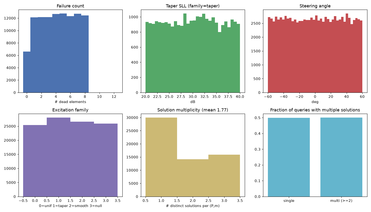
Metrics. Everything is scored on a fine 2001-point grid: beam-pointing error (degrees), PSLL degradation (how much the peak sidelobe worsened vs. target, dB), directivity loss (dB), pattern NMSE (dB domain), plus constraint-violation rate, sample diversity, and wall-time. Test sets: 1,000 i.i.d. held-out queries, and three out-of-distribution splits — heavier failure counts (10–12, trained on ≤8), wider steering (60–78°, trained on ≤60°), and held-out contiguous blocks.

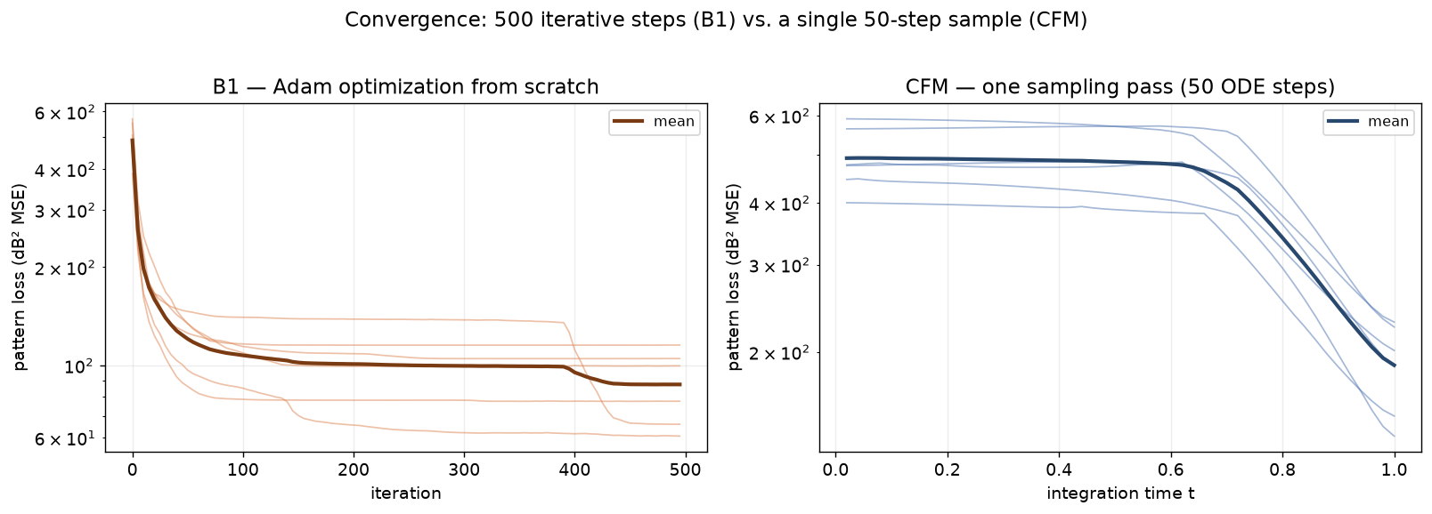
Optimization vs. generation. The two solvers reach an answer in completely different ways. B1 takes hundreds of iterative gradient steps from a random start; CFM takes one sampling pass. Here is that difference, on the same six random-failure queries:

Left: B1 grinds down the pattern loss over 500 Adam steps — and plateaus at very different levels per query (some get stuck high). Right: the CFM endpoint estimate's pattern loss collapses over a single 50-step integration, landing low and consistently.

4 · Results

Headline (i.i.d. test, n = 1000). Pointing error, PSLL degradation, directivity loss, dB-NMSE, constraint-violation rate:

method	pointing (°)	PSLL deg (dB)	dir. loss (dB)	NMSE	viol
B2 — deterministic regression	33.14	+8.09	1.20	1.689	0
B1 — from-scratch optimization	19.44	+12.56	2.54	0.728	0
CFM — best-of-8	0.433	+7.07	1.54	0.899	0
CFM — best-of-8 + polish	0.412	+7.17	1.79	0.542	0

You can see the difference in the reconstructed patterns. Black is the target; watch where each method puts the mainlobe:

Reconstructed patterns vs. target, at 2 / 4 / 8 random failures. B2 (red) and B1 (orange) routinely place the beam in the wrong direction; CFM (blue/green) locks onto the target mainlobe and tracks the near sidelobes.

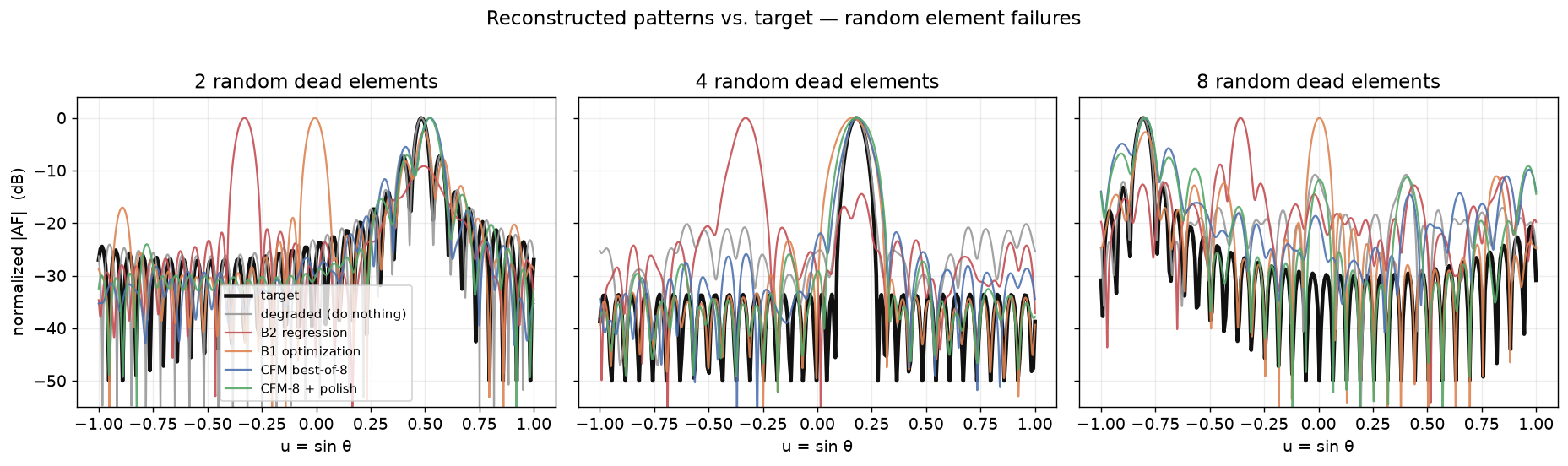
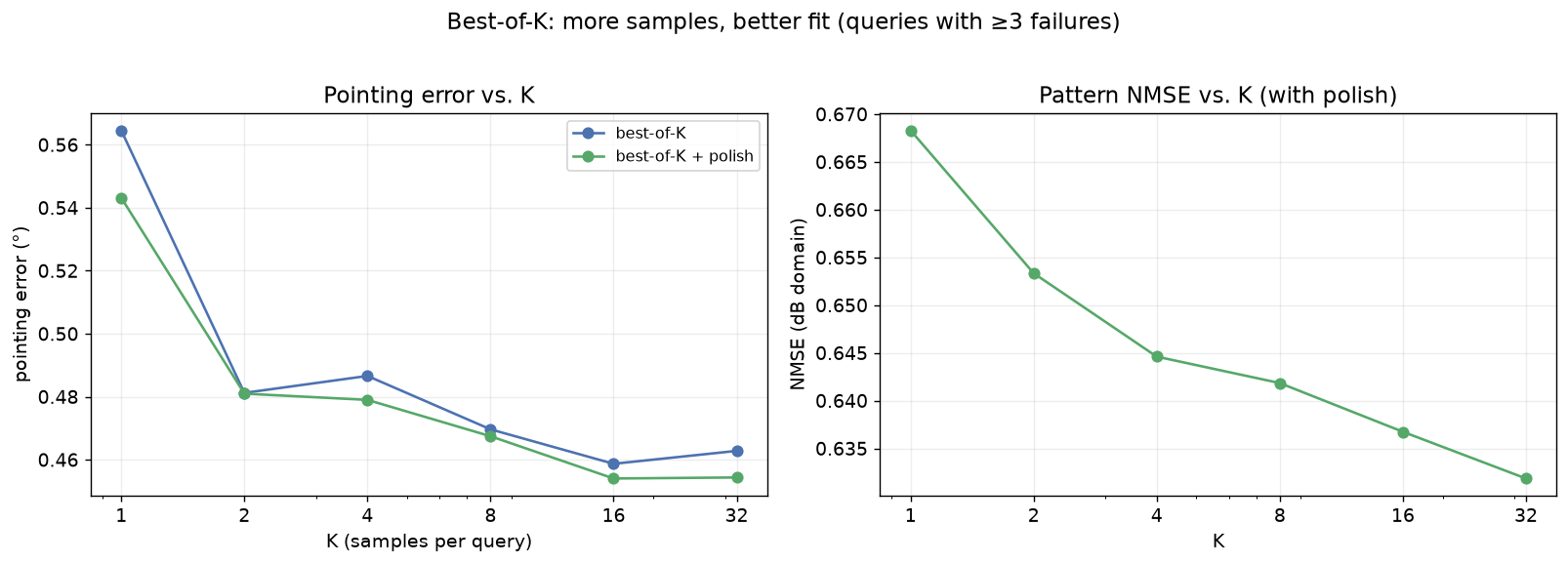
“Best-of-8” means: draw 8 samples, keep the one whose actual pattern best matches the target — cheap, because sampling batches on the GPU, and it only works because the samples genuinely differ. How performance scales with the number of samples K:

Best-of-K on queries with ≥3 failures. More samples steadily lower both pointing error and pattern NMSE — a knob you can turn at inference for more quality, entirely in parallel.

And the samples really are distinct solutions, not jitter around one answer:

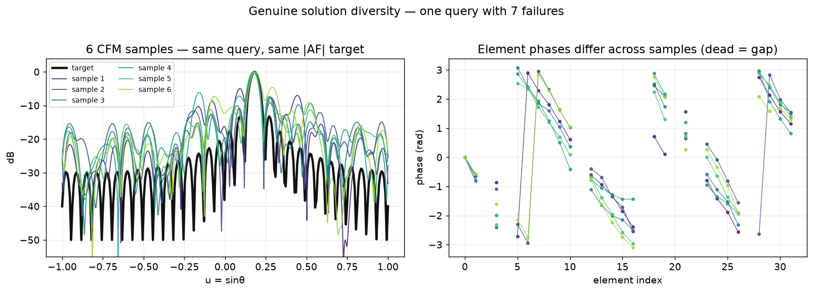
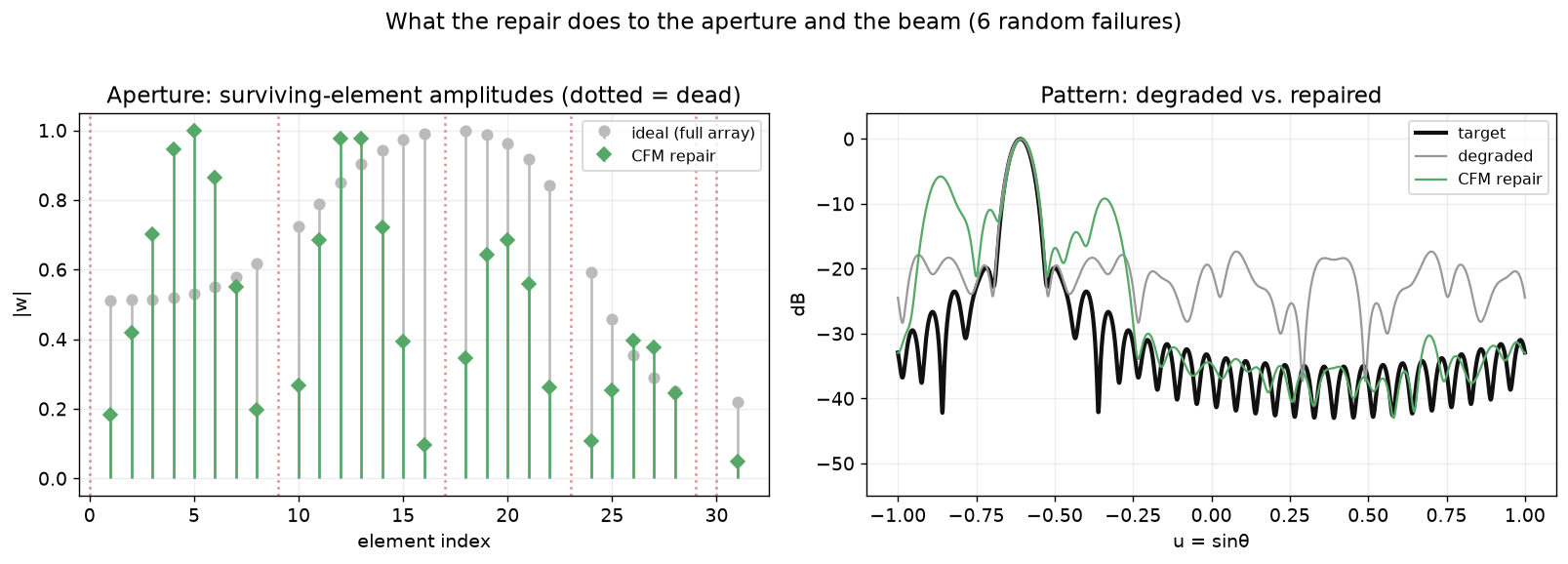
Six CFM samples for a single high-failure query. Left: all six reproduce the same target |AF|. Right: their per-element phases are genuinely different — different valid repairs, exactly the one-to-many structure. Across the test set, 82% of ≥4-failure queries yield ≥2 distinct repairs (target: 30%).

What a repair does concretely — which survivors it re-weights, and how the beam comes back:

A 6-random-failure case. Left: the CFM repair re-weights the surviving elements (dotted = dead). Right: the degraded beam (grey) vs. the CFM repair (green) against the target — the mainlobe and near sidelobes are restored.

Same query, both solvers, side by side — B1 optimizing from scratch on the left, CFM sampling on the right:

On a lucky query the from-scratch optimizer can look fine — but the live pointing readout gives it away, and across the test set B1 averages ~19° while CFM stays sub-degree. B1 also needs hundreds of iterative steps; CFM is one pass.

Out of distribution.

split	CFM-8+polish pointing (°)	PSLL deg (dB)	NMSE
i.i.d.	0.41	+7.2	0.54
contiguous-block failures (held out)	0.22	+4.6	0.24
10–12 failures (trained ≤ 8)	0.71	+10.7	1.33
steering 60–78° (trained ≤ 60°)	22.6	+3.8	0.78

5 · Analysis

Why the baselines fail at pointing. The metric-vs-failures curves make the mechanism plain:

Beam-pointing error (log scale, left) and PSLL degradation (right) vs. failure count. CFM (green) holds 0.1–0.6° pointing and the lowest sidelobe degradation across the whole range; B1 (orange) sits at 8–25°, B2 (red) flat near 35°.

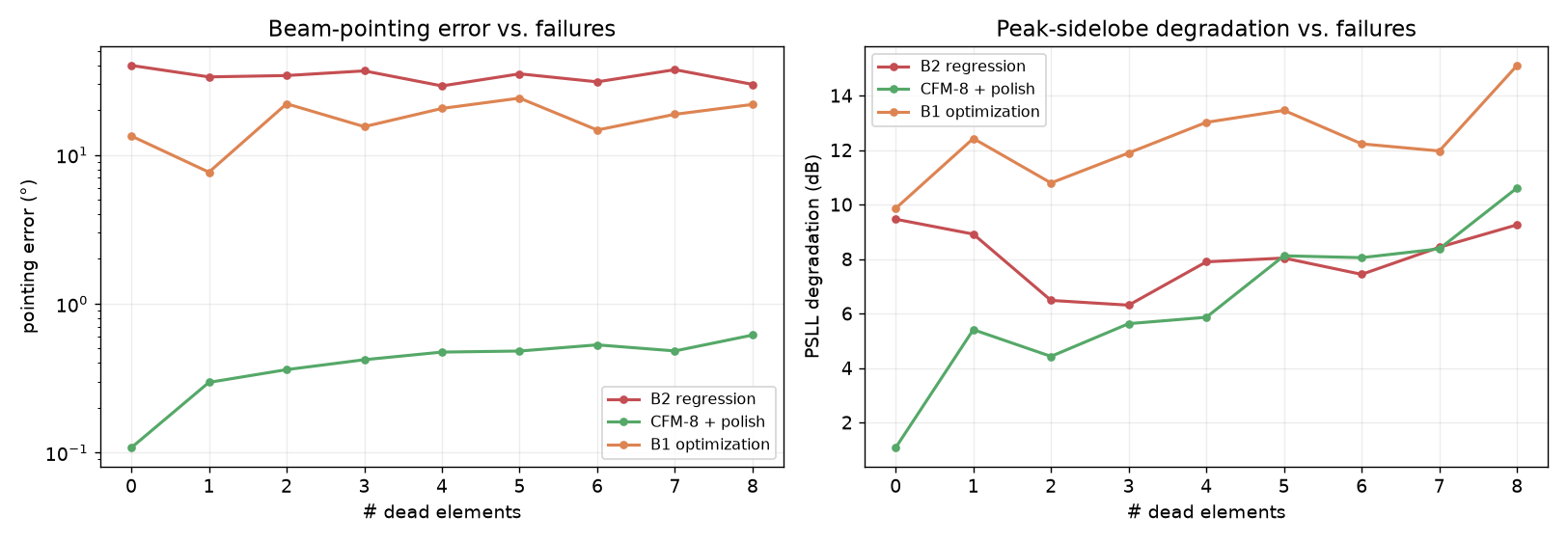
• B2 (regression) is flat at ~33° regardless of failures. It isn’t struggling with the failures — it’s averaging the modes. When several valid weight vectors exist, MSE regression pulls the prediction toward their mean, which points nowhere in particular. This is the exact pathology the generative framing exists to fix.
• B1 (optimization) sits at ~15–25° with huge variance. From a random start, magnitude-only repair is non-convex; the optimizer routinely settles into a basin whose |AF| looks plausible but whose mainlobe faces the wrong way. It can nail a lucky query (which is why single-example demos flatter it) and blow the next one.
• CFM’s learned prior fixes both. It has seen the solution manifold, so a single sample already lands near a valid mode, and best-of-K + polish sharpens it. The result — sub-degree pointing, lowest PSLL degradation, zero violations — is stronger than the target I set out for (“approach B1”); CFM beats both baselines.

Is it faster? It depends what you hold fixed, so I measured both.

method	single-query latency	achieved pointing
B1 (500 steps × 8 restarts)	247 ms	still ~14–20°
CFM-1	156 ms	0.47°
CFM-8	181 ms	0.39°

Per query CFM is both faster and far more accurate — and, crucially, B1 cannot buy CFM’s accuracy at any budget from a random start; it plateaus in a bad basin. CFM does a fixed ~100 network evals with no backprop, and best-of-K batches trivially.

Ablations.

change	pointing (°)	takeaway
physics regularizer ON	0.44	vs 0.53 off — it helps
Euler vs Heun (50 steps)	0.44 / 0.44	indistinguishable; Euler cheaper
20 sampling steps	0.45	already converged — 20 steps suffice
DPS guidance (η = 0.3)	3.63	hurts pointing as tuned — an honest negative

The guidance result is a useful reminder: a gradient nudge toward “lower pattern error” can quietly walk the beam off-target while improving average NMSE. Not every physics prior helps if you bolt it on carelessly.

Honest limitation. Steering angles beyond the training range are the real failure mode — every method degrades there (CFM 22.6°, B1 59°, B2 70°). Extrapolating the conditioning distribution is hard, and I’d rather report it than bury it.

6 · Stage B: the planar array

The same machinery generalizes to a 16×16 planar array — 256 elements, a 512-dimensional weight space, a 2-D pattern over direction cosines (u, v). The 2-D array factor factorizes into two matmuls, which is also how I killed an early memory blow-up: writing it as einsum("vn,...un->...uv") silently materializes a multi-gigabyte broadcast intermediate; two plain matmuls contract directly, ~5× faster and a fraction of the memory. (One other bug worth flagging for anyone doing this: my first 2-D pattern encoder used global average pooling, which throws away where the beam points — pointing error was stuck at 22° until I switched to a position-preserving head, which dropped it to 2.7°.)

Training a 2-D CFM on 17.6k planar repairs, on 800 held-out queries:

method	pointing (°)	PSLL deg (dB)	dir. loss (dB)	NMSE	viol
B1 — from-scratch optimization	41.9	+3.94	0.32	0.997	0
CFM — best-of-8	2.73	+4.00	1.41	2.008	0
CFM — best-of-8 + polish	2.73	+2.97	0.72	0.640	0

The 512-dimensional magnitude-only problem is genuinely harder, so pointing lands at ~2.7° rather than Stage A’s sub-degree — but that still beats from-scratch optimization by ~15× (B1 wanders to 41.9°, hopelessly stuck), keeps zero violations, and stays diverse (85% of ≥8-failure queries yield ≥2 distinct repairs). Here it is on both failure modes — a representative random-failure case and a held-out contiguous block:

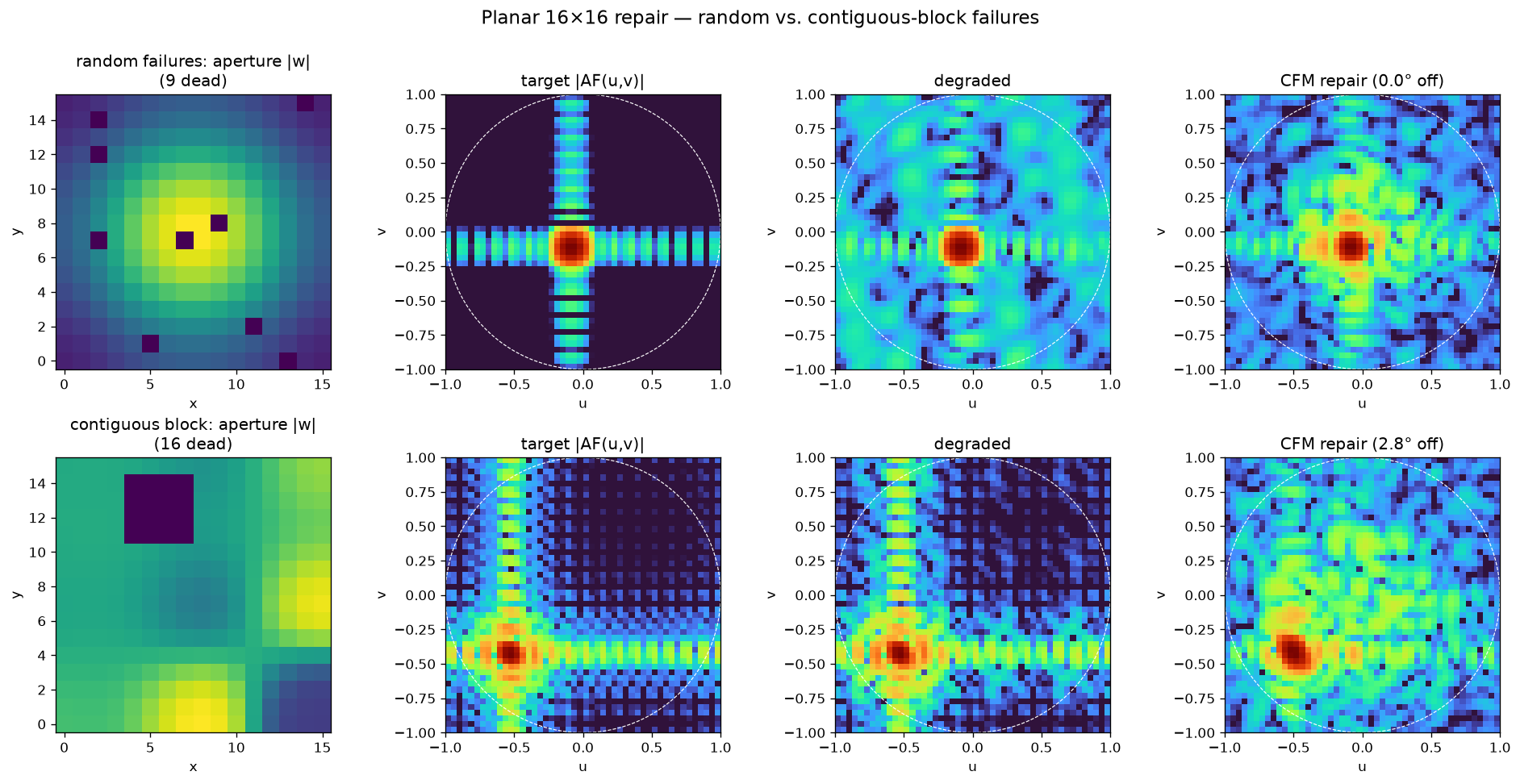
Planar 16×16 repair. Each row: the aperture (dark = dead), the target |AF(u,v)|, the degraded pattern, and the CFM repair. The dead 5×5 block (bottom) is compensated to 2.8°; a 9-random-failure case (top) to 0.0°.

The trained planar CFM sampling a repair from noise — this is generation, the learned model, not optimization:

Planar CFM sampling for a random-failure query: the 2-D far field condensing out of noise (left) toward the target (right) over the ODE integration.

For contrast, the same 2-D problem solved by direct optimization — aperture, achieved pattern, and target, descending the loss step by step (this one is not the learned model):

Direct (Adam) optimization of a planar block-failure repair — aperture with the dead 5×5 block, the achieved |AF(u,v)| reforming toward the target on the right.

---

Built in PyTorch on Apple-Silicon MPS. Forward model, dataset generator, baselines, the flow-matching model and its constrained sampler, the evaluation harness, and every figure/video here are custom. The one-to-many framing follows the conditional-flow-matching / rectified-flow line of work; the guided-sampling nudge is DPS-style.